Smart Systems, Inc. | Algorithms

Artificial Intelligence Algorithms

Artificial Intelligence algorithms uses an assortment of accurate, probabilistic, and upgraded techniques that empower computers to pick up from the past point of reference and perceive hard-to-perceive patterns from massive, noisy, or complex datasets. SSI uses the Algorithms outlined below to handle large and complex data to draw interesting patterns or trends in them such as anomalies. Machines are needed to process information fast and make decisions when it reaches the threshold.

Items	ML Algorithm Categories	ML Algorithms	Descriptions
1	Deep Learning	Deep Boltzmann Machine (DBM)	A deep Boltzmann machine is a model with more hidden layers with directionless connections between the nodes. DBM learns the features hierarchically from the raw data and the features extracted in one layer are applied as hidden variables as input to the subsequent layer.
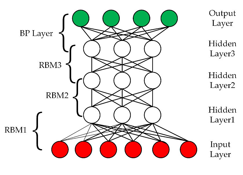
			Deep Belief Networks (DBN)	Deep Belief Networks are machine learning algorithm that resembles the deep neural network but are not the same. These are feedforward neural networks with a deep architecture. Simple, unsupervised networks like restricted Boltzmann machines or autoencoders make DBNs, with the hidden layer of each sub-network serving as the visible layer for the next layer.
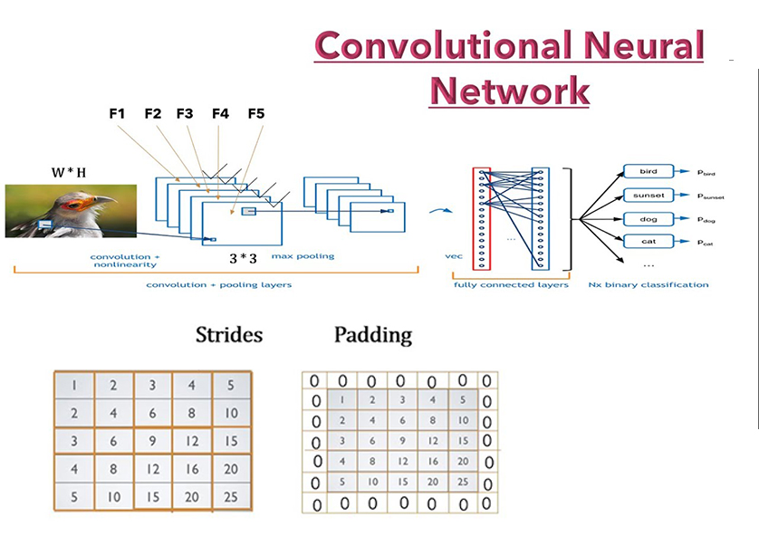
			Convolutional Neural Networks (CNN)	A convolutional neural network (CNN or convnet) is a subset of machine learning. It is one of the various types of artificial neural networks which are used for different applications and data types. A CNN is a kind of network architecture for deep learning algorithms and is specifically used for image recognition and tasks that involve the processing of pixel data.
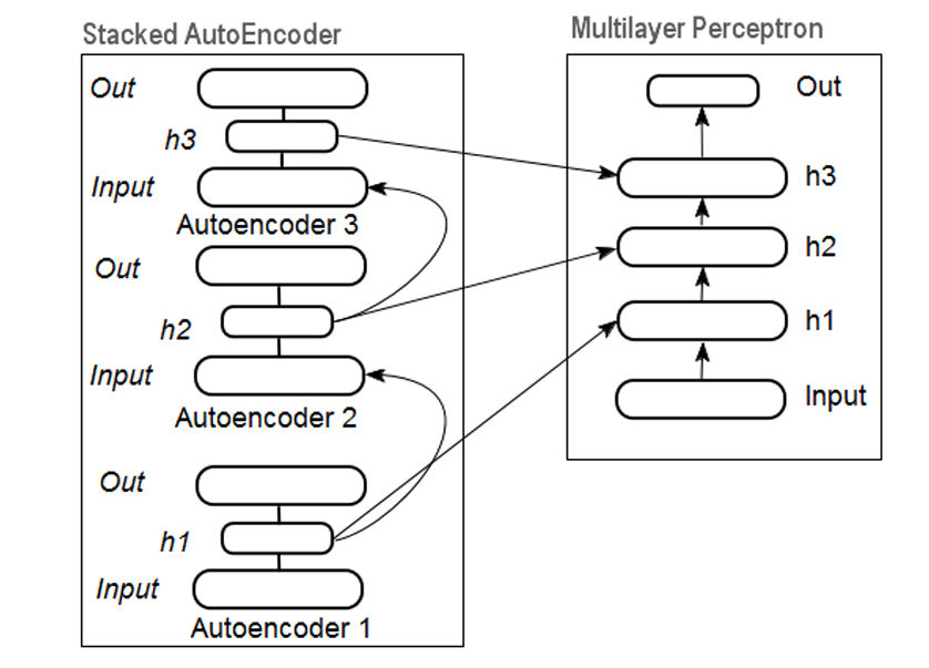
			Stacked Auto-Encoders	A stacked autoencoder is a multi-layer neural network that consists of multiple autoencoders, where the output of each encoder gets fed into the next encoder until the last encoder feeds its output into a chain of decoders. This allows a step by step compression and decompression of the input data to happen with more control over each state of the process.
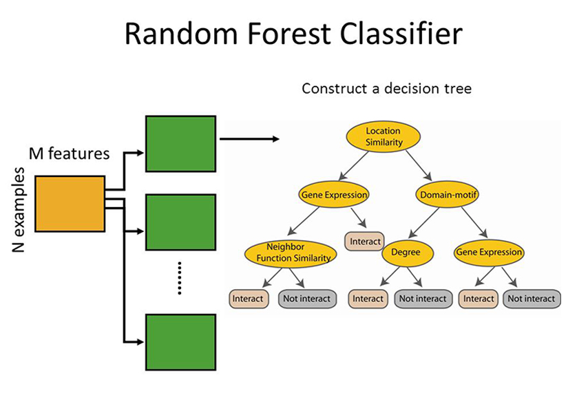
2	Ensemble	Random Forrest	Random forests or random decision forests is an ensemble learning method for classification, regression and other tasks that operates by constructing a multitude of decision trees at training time. For classification tasks, the output of the random forest is the class selected by most trees. For regression tasks, the mean or average prediction of the individual trees is returned
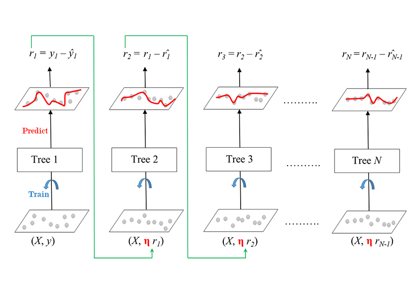
			Gradient Boosting Machine (GBM)	Gradient boosting is a machine learning technique used in regression and classification tasks, among others. It gives a prediction model in the form of an ensemble of weak prediction models, which are typically decision trees. When a decision tree is the weak learner, the resulting algorithm is called gradient-boosted trees; it usually outperforms random forest. A gradient-boosted trees model is built in a stage-wise fashion as in other boosting methods, but it generalizes the other methods by allowing optimization of an arbitrary differentiable loss function.
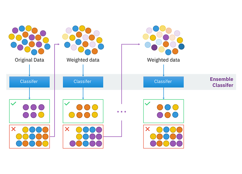
			Boosting	In machine learning, boosting is an ensemble meta-algorithm for primarily reducing bias, and also variance in supervised learning, and a family of machine learning algorithms that convert weak learners to strong ones. Boosting is based on the question posed by Kearns and Valiant (1988, 1989), "Can a set of weak learners create a single strong learner?" A weak learner is defined to be a classifier that is only slightly correlated with the true classification
			Bootstrapped Aggregation (Bagging)	Bootstrap aggregating, also called bagging, is a machine learning ensemble meta-algorithm designed to improve the stability and accuracy of machine learning algorithms used in statistical classification and regression. It also reduces variance and helps to avoid overfitting. Although it is usually applied to decision tree methods, it can be used with any type of method. Bagging is a special case of the model averaging approach.
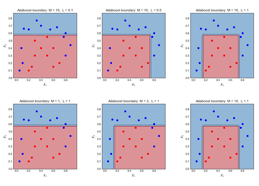
			AdaBoost	Adaptive Boosting, is a statistical classification meta-algorithm formulated by Yoav Freund and Robert Schapire in 1995, who won the 2003 Gödel Prize for their work. It can be used in conjunction with many other types of learning algorithms to improve performance. The output of the other learning algorithms ('weak learners') is combined into a weighted sum that represents the final output of the boosted classifier.
			Stacked Generalization (Blending)	Stacked Generalization is a general method of using a high-level model to combine lower- level models to achieve greater predictive accuracy.
			Gradient Boosted Regression Trees (GBRT)	Gradient Boosted Regression Trees (GBRT) or shorter Gradient Boosting is a flexible non-parametric statistical learning technique for classification and regression. This notebook shows how to use GBRT in scikit-learn, an easy-to-use, general-purpose toolbox for machine learning in Python.
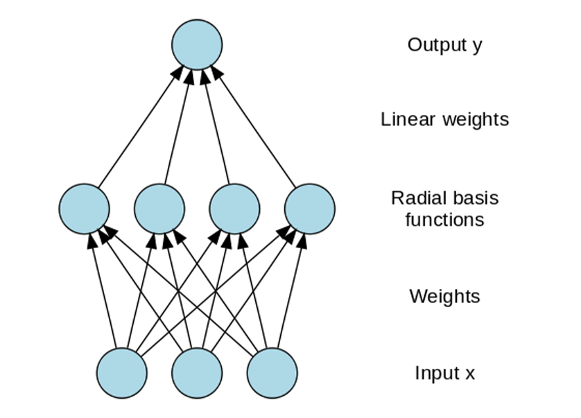
3	Neural Networks	Radial Basis Function Network (RBFN)	A radial basis function network is an artificial neural network that uses radial basis functions as activation functions. The output of the network is a linear combination of radial basis functions of the inputs and neuron parameters. Radial basis function networks have many uses, including function approximation, time series prediction, classification, and system control
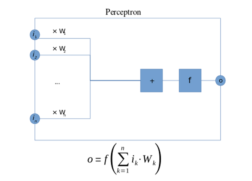
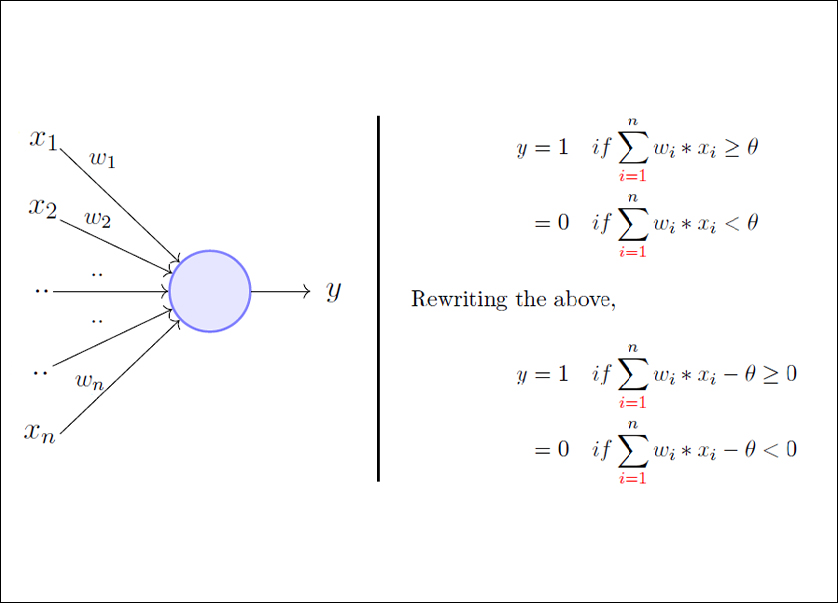
			Perceptron	A Perceptron is a neural network unit that does certain computations to detect features or business intelligence in the input data. It is a function that maps its input “x,” which is multiplied by the learned weight coefficient, and generates an output value ”f(x).
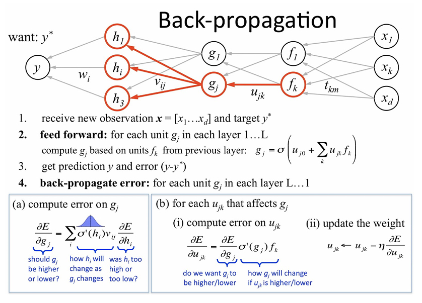
			Back-Propagation	Backpropagation is an algorithm used in artificial intelligence (AI) to fine-tune mathematical weight functions and improve the accuracy of an artificial neural network's outputs. A neural network can be thought of as a group of connected input/output (I/O) nodes.
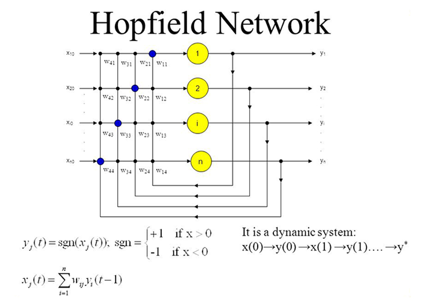
			Hopfield Network	A Hopfield network is a single-layered and recurrent network in which the neurons are entirely connected, i.e., each neuron is associated with other neurons. If there are two neurons i and j, then there is a connectivity weight wij lies between them which is symmetric wij = wji.
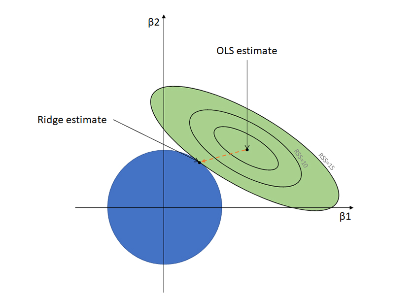
4	Regularization	Ridge Regression	Ridge regression is a model tuning method that is used to analyse any data that suffers from multicollinearity. This method performs L2 regularization. When the issue of multicollinearity occurs, least-squares are unbiased, and variances are large, this results in predicted values being far away from the actual values.
			Least Absolute Shrinkage and Selection Operator (LASSO)	The LASSO is an extension of OLS, which adds a penalty to the RSS equal to the sum of the absolute values of the non-intercept beta coefficients multiplied by parameter λ that slows or accelerates the penalty.
			Elastic Net	Elastic net linear regression uses the penalties from both the lasso and ridge techniques to regularize regression models. The technique combines both the lasso and ridge regression methods by learning from their shortcomings to improve the regularization of statistical models.
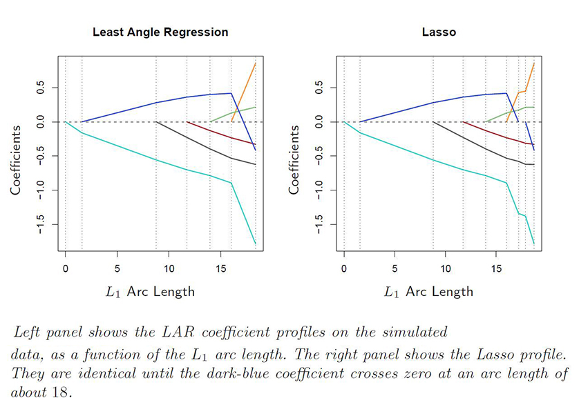
			Least Angle Regression (LARS)	Least-Angle Regression (LARS) is an algorithm for fitting linear regression models to high-dimensional data, developed by Bradley Efron, Trevor Hastie, Iain Johnstone and Robert Tibshirani.
5	Rule System	Cubist	Cubist is a rule-based model that is an extension of Quinlan's M5 model tree. A tree is grown where the terminal leaves contain linear regression models. These models are based on the predictors used in previous splits. Also, there are intermediate linear models at each step of the tree.
			One Rule (OneR)	OneR, short for "One Rule", is a simple, yet accurate, classification algorithm that generates one rule for each predictor in the data, then selects the rule with the smallest total error as its "one rule". To create a rule for a predictor, we construct a frequency table for each predictor against the target.
			Zero Rule (ZeroR)	Zero Rule or ZeroR is the benchmark procedure for classification algorithms whose output is simply the most frequently occurring classification in a set of data. If 65% of data items have that classification, ZeroR would presume that all data items have it and would be right 65% of the time.
			Repeated Incremental Pruning to Produce Error Reduction (RIPPER)	The Ripper Algorithm is a Rule-based classification algorithm. It derives a set of rules from the training set. It is a widely used rule induction algorithm.
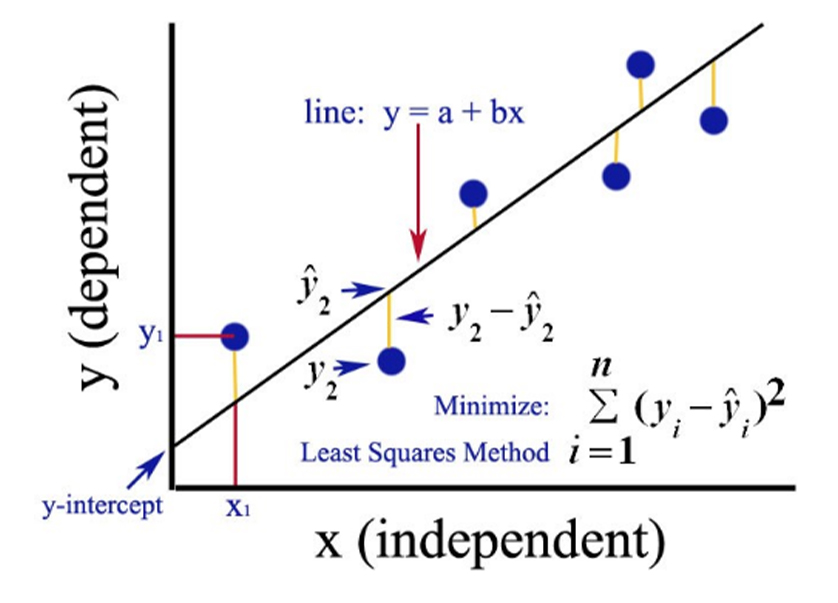
6	Regression	Linear Regression	Linear regression is a linear approach for modelling the relationship between a scalar response and one or more explanatory variables. The case of one explanatory variable is called simple linear regression; for more than one, the process is called multiple linear regression.
			Ordinary Least Square Regression (OLSR)	Ordinary Least Squares Regression (OLS) is a common technique for estimating coefficients of linear regression equations which describe the relationship between one or more independent quantitative variables and a dependent variable (simple or multiple linear regression).
			Stepwise Regression	Stepwise Regression is a method of fitting regression models in which the choice of predictive variables is carried out by an automatic procedure. In each step, a variable is considered for addition to or subtraction from the set of explanatory variables based on some prespecified criterion.
			Multivariate Adaptive Regression Splines (MARS)	Multivariate adaptive regression splines (MARS) is a form of regression analysis introduced by Jerome H. Friedman in 1991. It is a non-parametric regression technique and can be seen as an extension of linear models that automatically models nonlinearities and interactions between variables.
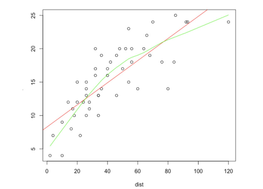
			Locally Estimated Scatterplot Smoothing (LOESS)	Locally Estimated Scatterplot Smoothing, or LOESS, is a nonparametric method for smoothing a series of data in which no assumptions are made about the underlying structure of the data. LOESS uses local regression to fit a smooth curve through a scatterplot of data.
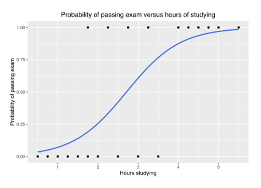
			Logistics Regression	The logistic model is a statistical model that models the probability of an event taking place by having the log-odds for the event be a linear combination of one or more independent variables. In regression analysis, logistic regression is estimating the parameters of a logistic model.
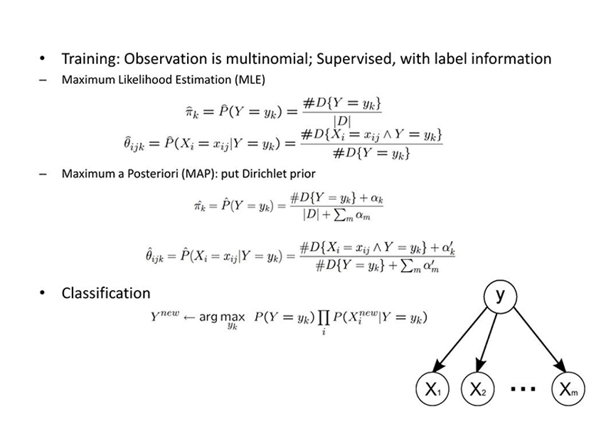
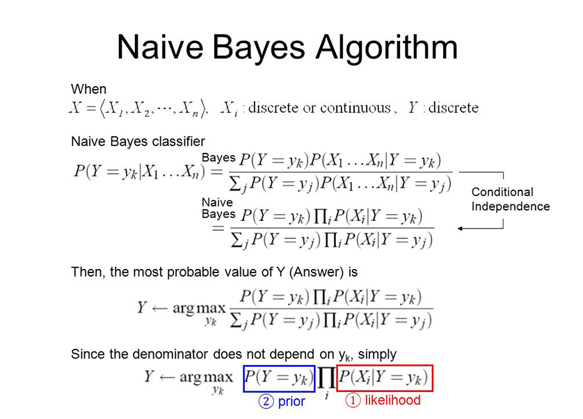
7	Bayesian	Naïve Bayes	Naïve Bayes is a simple learning algorithm that utilizes Bayes rule together with a strong assumption that the attributes are conditionally independent, given the class. While this independence assumption is often violated in practice, naïve Bayes nonetheless often delivers competitive classification accuracy.
			Averaged one-Dependence Estimators (AODE)	Averaged one-dependence estimators is a semi-naive Bayesian Learning method. It performs classification by aggregating the predictions of multiple one-dependence classifiers in which all attributes depend on the same single parent attribute as well as the class.
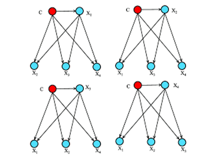
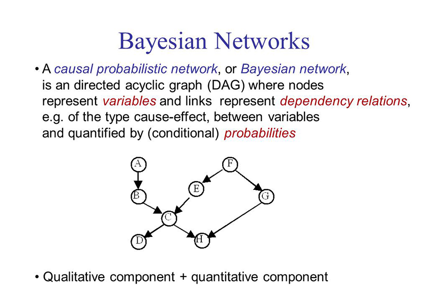
			Bayesian Belief Network (BBN)	Bayesian Belief Network (BBN) is a Probabilistic Graphical Model (PGM) that represents a set of variables and their conditional dependencies via a Directed Acyclic Graph (DAG). To understand what this means, let's draw a DAG and analyze the relationship between different nodes.
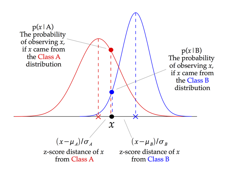
			Gaussian Naïve Bayes	Gaussian Naive Bayes assumes that each class follow a Gaussian distribution. The difference between QDA and (Gaussian) Naive Bayes is that Naive Bayes assumes independence of the features, which means the covariance matrices are diagonal matrices.
			Multinomial Naïve Bayes	The Multinomial Naive Bayes algorithm is a Bayesian learning approach popular in Natural Language Processing (NLP). The program guesses the tag of a text, such as an email or a newspaper story, using the Bayes theorem. It calculates each tag's likelihood for a given sample and outputs the tag with the greatest chance.
			Bayesian Network (BN)	A Bayesian network (BN) is a probabilistic graphical model for representing knowledge about an uncertain domain where each node corresponds to a random variable and each edge represents the conditional probability for the corresponding random variables [9]. BNs are also called belief networks or Bayes nets.
8	Decision Tree	Classification and Regression Tree (CART)	A Classification And Regression Tree (CART), is a predictive model, which explains how an outcome variable's values can be predicted based on other values. A CART output is a decision tree where each fork is a split in a predictor variable and each end node contains a prediction for the outcome variable.
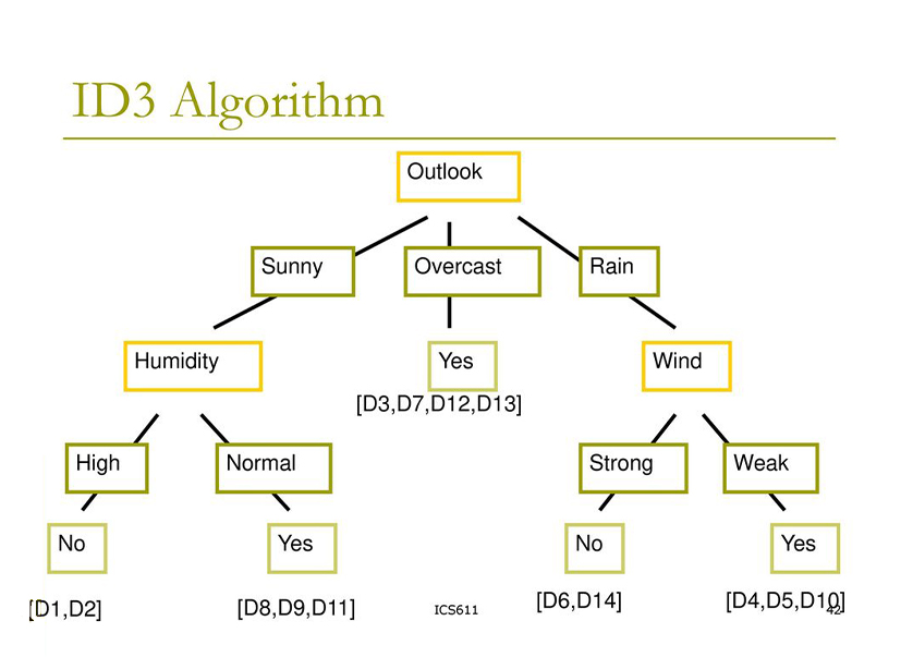
			Iterative Dichotomiser 3 (ID3)	ID3 (Iterative Dichotomiser 3) is an algorithm invented by Ross Quinlan used to generate a decision tree from a dataset. ID3 is the precursor to the C4. 5 algorithm, and is typically used in the machine learning and natural language processing domains.
			C4.5	5 is an algorithm used to generate a decision tree developed by Ross Quinlan. C4. 5 is an extension of Quinlan's earlier ID3 algorithm. The decision trees generated by C4.
			C5.0	A C5. 0 model works by splitting the sample based on the field that provides the maximum information gain . Each sub-sample defined by the first split is then split again, usually based on a different field, and the process repeats until the subsamples cannot be split any further.
			Chi-Squared Automatic Interaction Detection (CHAID)	Chi-square Automatic Interaction Detector (CHAID) was a technique created by Gordon V. Kass in 1980. CHAID is a tool used to discover the relationship between variables. CHAID analysis builds a predictive medel, or tree, to help determine how variables best merge to explain the outcome in the given dependent variable.
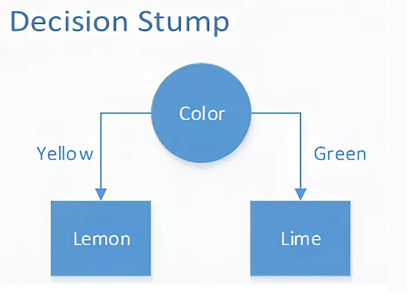
			Decision Stump	A decision stump is a machine learning model consisting of a one-level decision tree. That is, it is a decision tree with one internal node (the root) which is immediately connected to the terminal nodes (its leaves). A decision stump makes a prediction based on the value of just a single input feature.
			Conditional Decision Trees	Conditional Inference Trees is a different kind of decision tree that uses recursive partitioning of dependent variables based on the value of correlations. It avoids biasing just like other algorithms of classification and regression in machine learning.
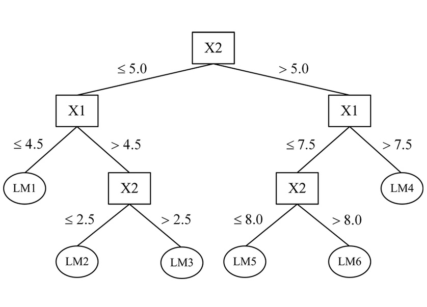
			M5	M5 model tree is a decision tree learner for regression task which is used to predict values of numerical response variable Y [13], which is a binary decision tree having linear regression functions at the terminal (leaf) nodes, which can predict continuous numerical attributes.
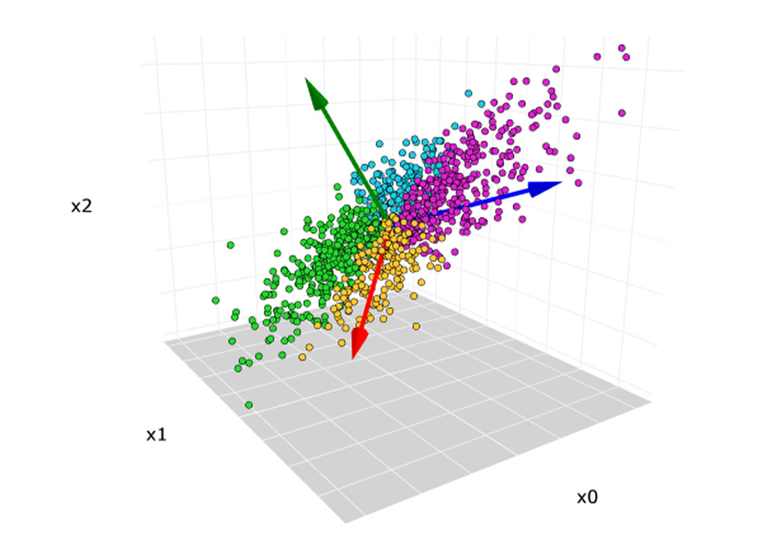
9	Dimensionality Reduction	Principal Component Analysis (PCA)	Principal component analysis (PCA) is a technique for reducing the dimensionality of such datasets, increasing interpretability but at the same time minimizing information loss. It does so by creating new uncorrelated variables that successively maximize variance.
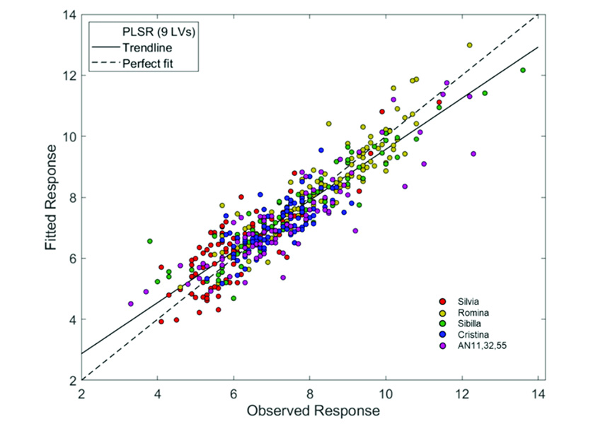
			Partial Least Squares Regression (PLSR)	The Partial Least Squares regression (PLS) is a method which reduces the variables, used to predict, to a smaller set of predictors. These predictors are then used to perfom a regression. Some programs differentiate PLS 1 from PLS 2. PLS 1 corresponds to the case where there is only one dependent variable.
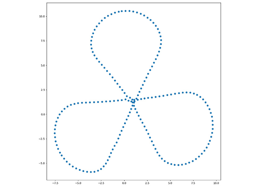
			Sammon Mapping	Sammon mapping or Sammon projection is an algorithm that maps a high-dimensional space to a space of lower dimensionality (see multidimensional scaling) by trying to preserve the structure of inter-point distances in high-dimensional space in the lower-dimension projection.
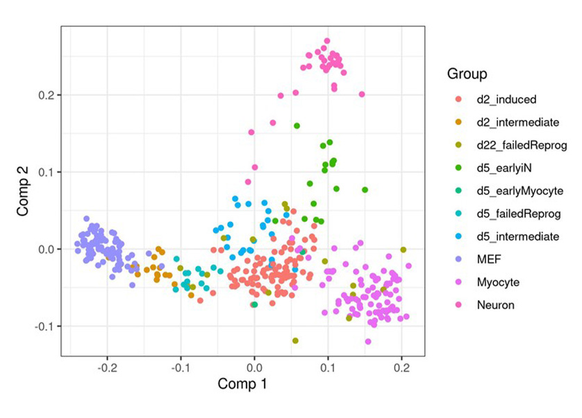
			Multidimensional Scalling (MDS)	Multidimensional scaling (MDS) is a means of visualizing the level of similarity of individual cases of a dataset. MDS is used to translate "information about the pairwise 'distances' among a set of objects or individuals" into a configuration of. points mapped into an abstract Cartesian space.
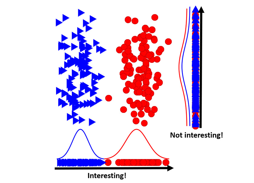
			Projection Pursuit	Projection pursuit (PP) is a type of statistical technique which involves finding the most "interesting" possible projections in multidimensional data. Often, projections which deviate more from a normal distribution are considered to be more interesting.
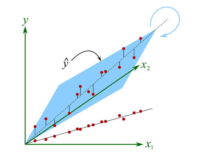
			Principal Component Regression (PCR)	Principal component regression (PCR) is a regression analysis technique that is based on principal component analysis (PCA). More specifically, PCR is used for estimating the unknown regression coefficients in a standard linear regression model.
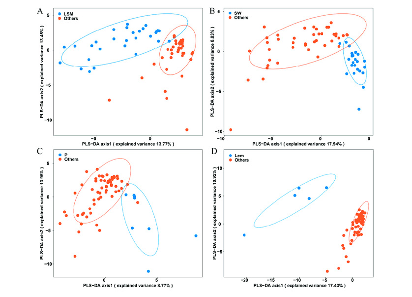
			Partial Least Squares Discriminant Analysis (PLSR)	Partial least squares-discriminant analysis (PLS-DA) is a versatile algorithm that can be used for predictive and descriptive modelling as well as for discriminative variable selection.
			Mixture Discriminant Analysis (MDA)	The LDA classifier assumes that each class comes from a single normal (or Gaussian) distribution. This is too restrictive. For MDA, there are classes, and each class is assumed to be a Gaussian mixture of subclasses, where each data point has a probability of belonging to each class.
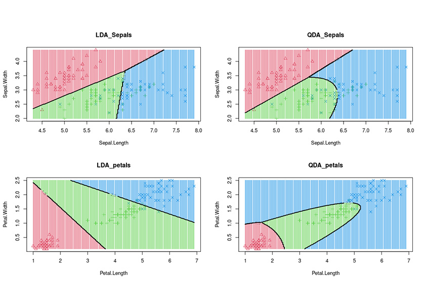
			Quadratic Discriminant Analysis (QDA)	Quadratic Discriminant Analysis (QDA) is a generative model. QDA assumes that each class follow a Gaussian distribution. The class-specific prior is simply the proportion of data points that belong to the class. The class-specific mean vector is the average of the input variables that belong to the class.
			Regularized Discriminant Analysis (RDA)	The regularized discriminant analysis (RDA) is a generalization of the linear discriminant analysis (LDA) and the quadratic discreminant analysis (QDA). Both algorithms are special cases of this algorithm. If the alpha parameter is set to 1, this operator performs LDA.
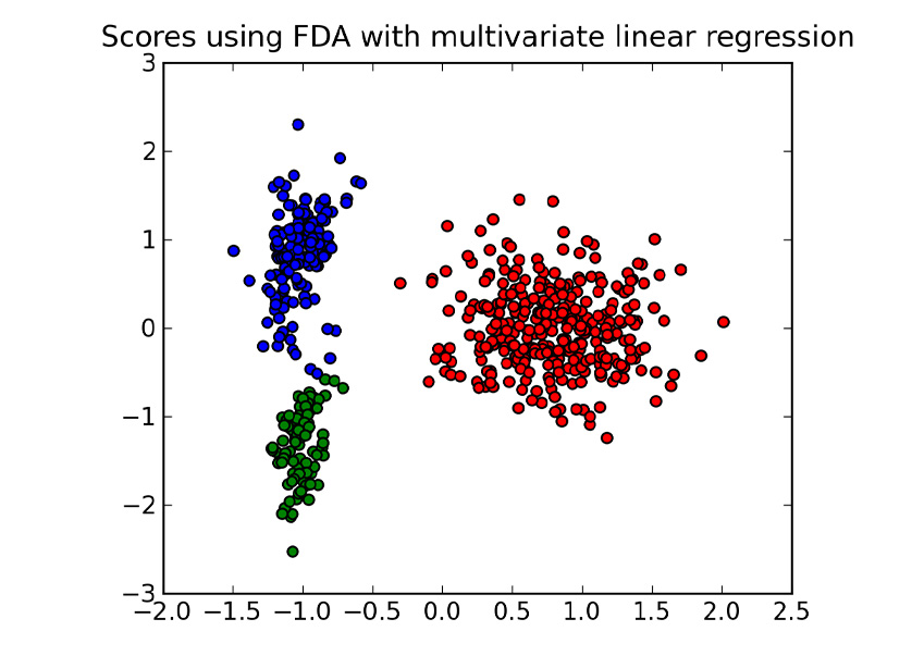
			Flexible Discriminant Analysis (FDA)	Flexible Discriminant Analysis is a classification model based on a mixture of linear regression models, which uses optimal scoring to transform the response variable so that the data are in a better form for linear separation, and multiple adaptive regression splines to generate the discriminant surface.
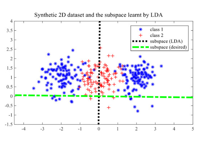
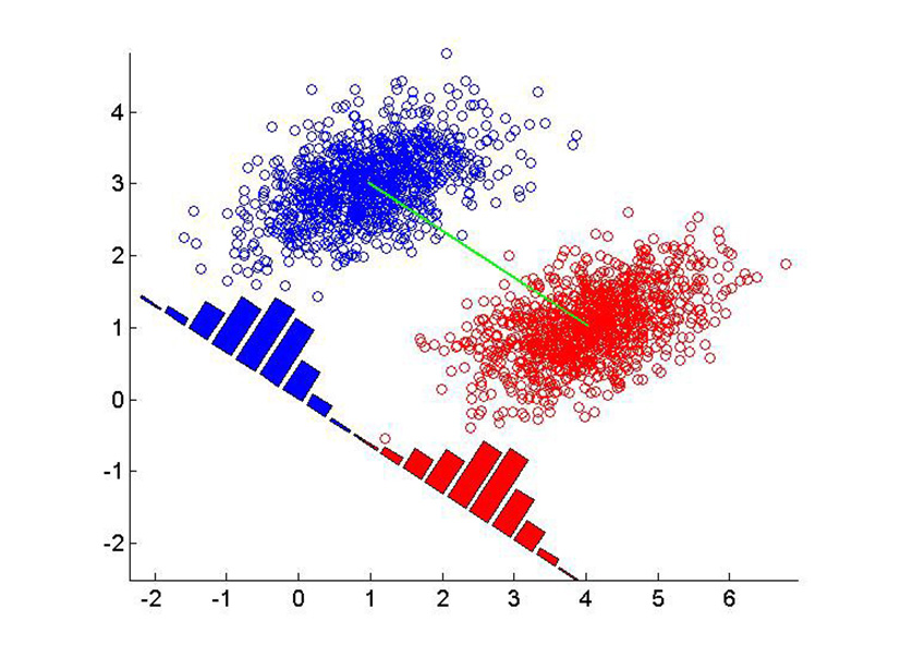
			Linear Discriminant Analysis (LDA)	Linear discriminant analysis (LDA), normal discriminant analysis (NDA), or discriminant function analysis is a generalization of Fisher's linear discriminant, a method used in statistics and other fields, to find a linear combination of features that characterizes or separates two or more classes of objects or events.
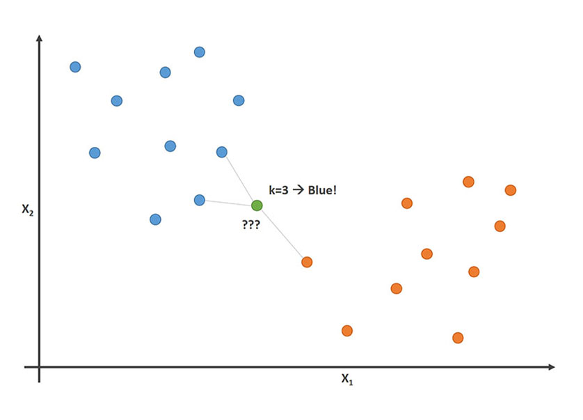
10	Instance Based	K-nearest Neighbour (KNN)	The k-nearest neighbors algorithm, also known as KNN or k-NN, is a non-parametric, supervised learning classifier, which uses proximity to make classifications or predictions about the grouping of an individual data point.
			Learning Vector Quantization (LVQ)	Learning Vector Quantization ( or LVQ ) is a type of Artificial Neural Network which also inspired by biological models of neural systems. It is based on prototype supervised learning classification algorithm and trained its network through a competitive learning algorithm similar to Self Organizing Map.
			Self-Organization Map (SOM)	Self Organizing Map (or Kohonen Map or SOM) is a type of Artificial Neural Network which is also inspired by biological models of neural systems from the 1970s. It follows an unsupervised learning approach and trained its network through a competitive learning algorithm.
			Locally Weighted Learning (LWL)	Locally Weighted Learning is a class of function approximation techniques, where a prediction is done by using an approximated local model around the current point of interest. This paper gives an general overview on the topic and shows two different solution algorithms.
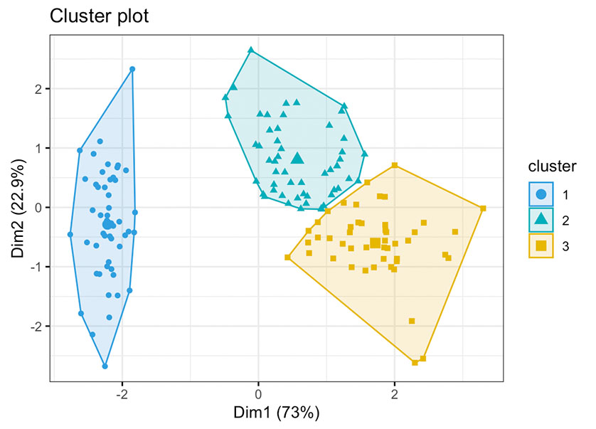
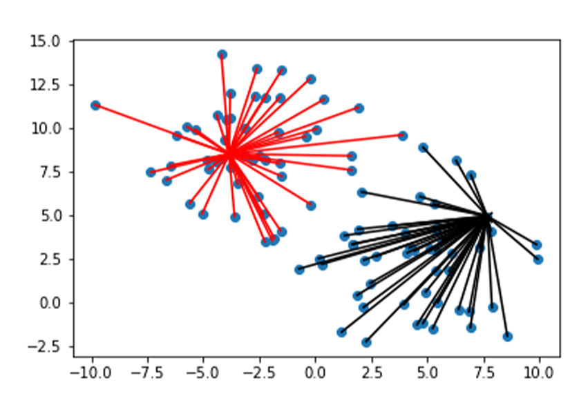
11	Clustering	K-means	k-means clustering is a method of vector quantization, originally from signal processing, that aims to partition n observations into k clusters in which each observation belongs to the cluster with the nearest mean (cluster centers or cluster centroid), serving as a prototype of the cluster.
			K-medians	K-medians is a clustering algorithm similar to K-means. K-medians and K-means both partition n observations into K clusters according to their nearest cluster center. In contrast to K-means, while calculating cluster centers, K-medians uses medians of each feature instead of means of it.
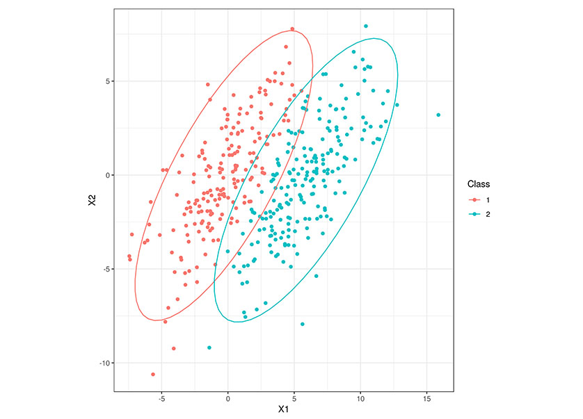
			Expectation Maximization	An expectation–maximization algorithm is an iterative method to find maximum likelihood or maximum a posteriori estimates of parameters in statistical models, where the model depends on unobserved latent variables.
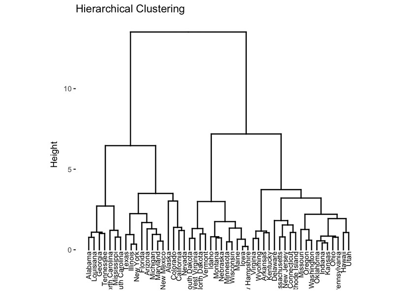
			Hierarchical Clustering	A Hierarchical clustering method works via grouping data into a tree of clusters. Hierarchical clustering begins by treating every data point as a separate cluster. Then, it repeatedly executes the subsequent steps: Identify the 2 clusters which can be closest together, and. Merge the 2 maximum comparable clusters.

These descriptions were extracted from reputable academic institutions and research organization that concentrate on AI technologies, and were vetted for accuracy and completeness before inclusion in the table above.

Artificial Intelligence Algorithms

Request a Quote or Demo